Function cardiac analysis mode

8.1 Function cardiac analysis mode

____________________________________________________________________________________________

Functionality is available in a separate module which is activated in the Pro edition for an extra fee
____________________________________________________________________________________________

8.1.1 Opening Studies for the Function Cardiac Analysis

To open a study for the function cardiac analysis, proceed as follows:

Choose a study and select MR series with images oriented along the short and long axis of the heart.In some cases, you don’t have to select series with images oriented along the long axis of the heart. For details on selecting series, see Section 1.10.
Click the Cardiac analysis button on the toolbar. To select the tab location (in the current window, in a separate window, or in the full-screen mode), press the arrow on the right-hand side of the button. To open the cardiac analysis window in a new tab in the current window, press the button. The process may take some time.
The Cardiac analysis tool is also available in the View section of the main menu.

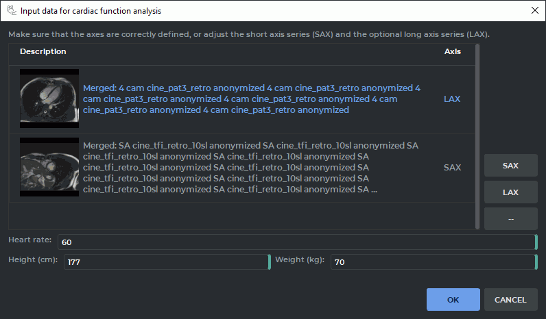
When the cardiac analysis module is activated, the Input data for cardiac analysis dialog box pops up (see Fig. 8.1). From the drop-down list, select the Function analysis mode. This mode provides for analysis and evaluation of cardiac functional parameters.

The T1 analysis mode provides an opportunity to create a map showing the T1 relaxation time for quantiﬁcation of changes in the cardiac tissue. For details on this mode, see Section 8.2.1.

In theFunction analysis mode, the DICOM Viewer automatically arranges the selected series in groups. A group consists of one or several series united by planes parallelism. If there is more than one series in a group, series are merged. For each series group, the type is automatically deﬁned: with images oriented along the short axis of the heart SAX (Short axis series) or with images oriented along the long axis of the heart LAX (Long axis series). Sometimes the series type cannot be deﬁned automatically. In this case, you will see the — symbol as the axis type.

If the series to be merged have the same names, a suﬃx (xN) will be added to the merged series description for each group of series with the same names, where N stands for the number of series with the same names.

Figure 8.1: "Input data for cardiac analysis" dialog box

The user may change the type of axis for the group. To do that, select the group and click the Set as SAX or Set as LAX button. You don’t need the series with images oriented along the long axis of the heart (LAX) series to analyze certain cardiac functions.

To reset the type of axis for the group, select it on the list and click Reset selected series — .

To continue work, you need at least one series or group to have the SAX type of axis.

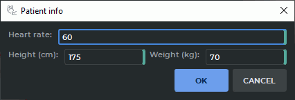
In the lower part of the dialog box, you can see the information about the patient that is loaded automatically. Sometimes only a part of the information is ﬁlled in automatically. In this case, other parameters referring to the patient must be provided manually:
- heart rate (beats/min);
- height (cm);
- weight (kg).
Click OK to enter the data required for cardiac function analysis or CANCEL to cancel.

If you haven’t provided all the required parameters in the Input data for cardiac analysis dialog box (see Fig. 8.1), the OK button will be deactivated.

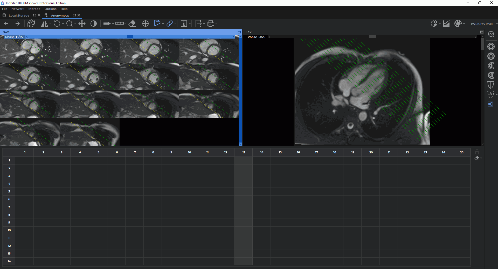
In the Cardiac analysis tab, you can see two windows, with the SAX merged series and the LAX merged series (Fig. 8.2). The toolbar for cardiac function analysis is on the right-hand side of the tab.

Under the SAX and LAX windows, you can see the contours panel aimed for navigation between images and contour management (for details see Section 8.1.7). By default, the panel is expanded.

Figure 8.2: Cardiac analysis tab

By default, all the slices for the current phase are shown in the SAX window. The phases may be switched by moving the slider along the horizontal scroll bar at the top of the SAX window or on the contour panel.

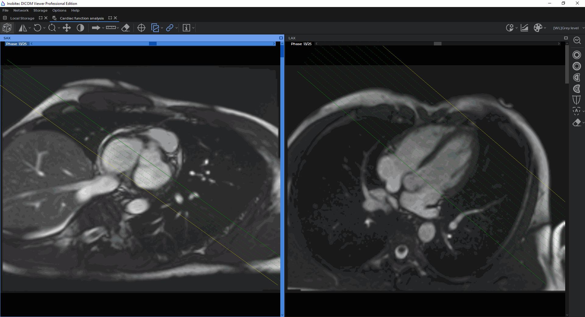
To escape the mode displaying all the slices for the current phase, click the right mouse button in the SAX window and disable the Multi-SAX arrangement option on the context menu. By default, the option is enabled and highlighted with blue on the menu. The SAX window in the Cardiac analysis tab will be displayed as shown in Fig. 8.3.

In this particular case, the SAX window shows only one slice for the current phase. The slices may be switched by moving the slider along the vertical scroll bar on the right-hand side of the window or on the contour panel.

Figure 8.3: The Multi-SAX arrangement option is disabled

To go back to the mode displaying all the slices for the current phase, click the right mouse button in the SAX window and enable the Multi-SAX arrangement option on the context menu.

If only one slice is displayed in the SAX window, the Multi-SAX arrangement option is unavailable.

After the slices are moved or scaled, their arrangement in the SAX window can be optimized. To do this, click the right mouse button in the SAX window and select the Apply auto transform option on the context menu. The slices arrangement in the SAX window will be optimized: the empty space will be minimized, and the heart will occupy the optimal position.

Slices arrangement optimization in the SAX window is applied by default when the Cardiac analysis tab is opened.

8.1.2 Tools for Cardiac Function Analysis

The toolbar for cardiac function analysis is on the right-hand side of the Cardiac analysis (Fig. 8.3).

Tools:

	The Endocardial LV contour button is aimed for building and editing the inner contour of the left ventricle manually (the contour is shown in red)
	The Epicardial LV contour button is aimed for building and editing the outer contour of the left ventricle manually (the contour is shown in yellow)
	The Endocardial RV contour button is aimed for building and editing the inner contour of the right ventricle manually (the contour is shown in dark-blue)
	The Epicardial RV contour button is aimed for building and editing the outer contour of the right ventricle manually (the contour is shown in light-blue)
	The LV extension boundaries button is aimed for manual determination of the left ventricle extension boundaries along the long axis (see Section 8.1.4)
	The Auto contouring button activates the process of automatic contouring of the left ventricle endocardium end epicardium (see Section 8.1.5)
	The Contours panel button is used to expand/minimize the contours panel that is used for navigation between images and for contour management (see Section 8.1.7)
	The Start analysis button triggers the analysis process and opens a panel with all the results of functional parameters evaluation (see Section 8.1.8)
	The Edit button closes the panel with the results and opens the toolbar for cardiac function analysis to provide an opportunity to build and edit contours

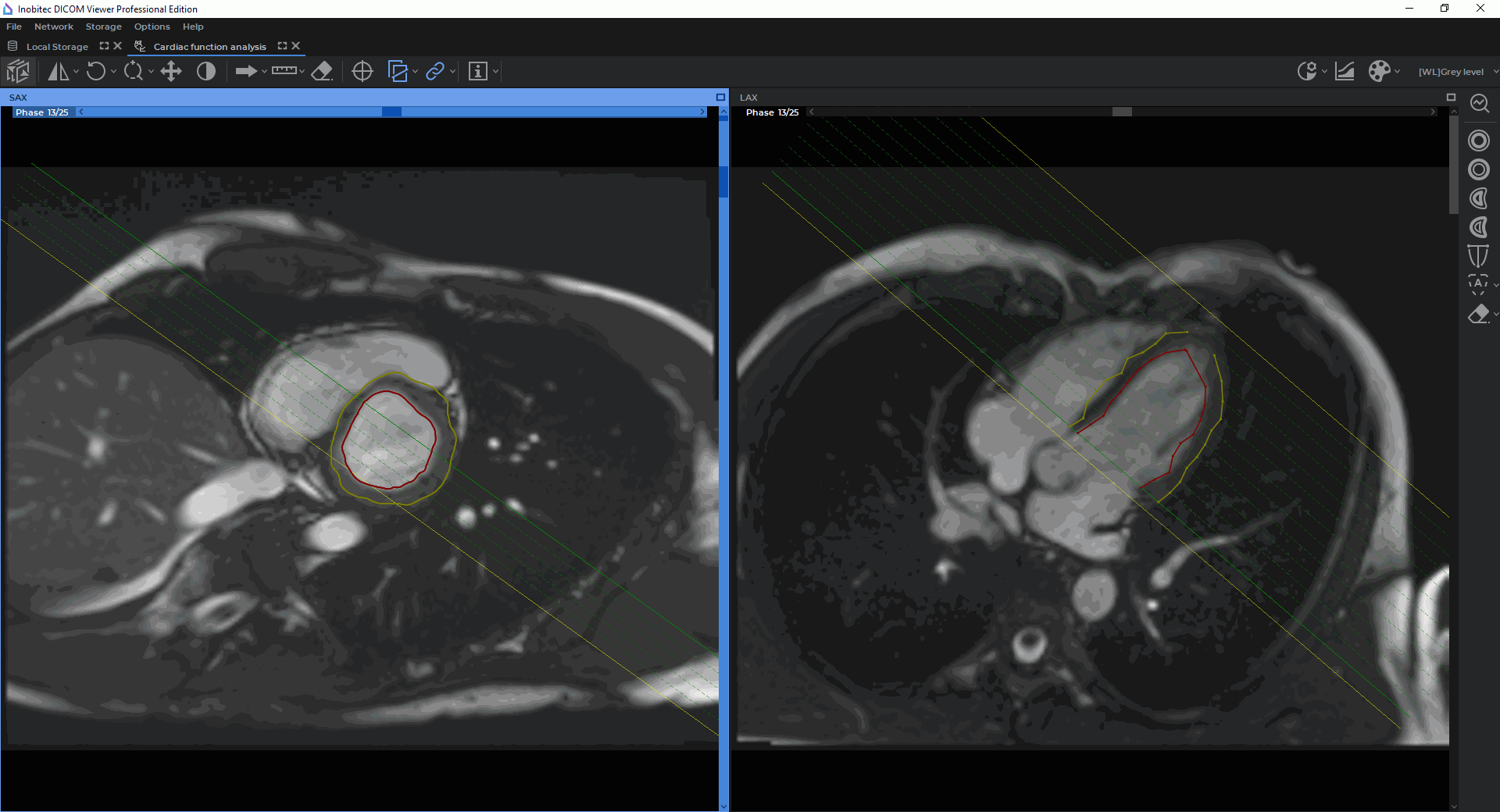
The functional parameters of the left and the right ventricles are calculated on the basis of the contours built. Contours can be built separately for each slice and phase in the window with the SAX merged series. The contour boundaries are shown as points on the slices in the window with the merge LAX series. If two or more contours were built for one phase, the points can be connected by segments. You cannot build contours in the window with a LAX merged series.

To simplify the process of building contours, we recommend enabling the display of slices scout lines in the window selected (see Section 2.26).

8.1.3 Building Contours Manually

You can use the following tools to build contours manually:

Endocardial LV contour ;
Epicardial LV contour ;
Endocardial RV contour ;
Epicardial RV contour .

The choice of the tool depends on the region of interest and the results of the analysis required.

To build a contour, proceed as follows:

Open the study in the Cardiac analysis tab (see Section 8.1.1).
Activate one of the contour building tools with the left, right, or middle mouse button. To continue work with the same tool, use the button with which the tool was activated. For details on tool management, see Section 1.14. Build the contour in one of the following ways:
- building contours manually. In the window with the SAX merged series, build a contour around the selected area while holding the button with which the tool was activated. To complete the contour, release the mouse button. To cancel the contour that has not been closed, click Esc on the keyboard while holding the mouse button;
- building contours with an isoline. Move the cursor around the selected area while holding the Shift button on the keyboard and the mouse button with which the tool was activated. Under the cursor, you will see an isoline. You can see an isoline only on the slices where a contour can be built. To build a contour with an isoline, release the mouse button with which the tool was activated.
Go to the next slice and contour the selected area.
After you have built the required contours, click the Start analysis button to go to the results of parameters assessment (see Section 8.1.8).

Figure 8.4: The Left ventricle epicardium and endocardium contours are shown in the SAX window, and the contour boundaries on the slices are shown in the LAX window

If there is a contour built with the current tool on the current slice, you cannot build a new contour here. You can only edit or delete the existing contour (see Section 8.1.6).

8.1.4 Evaluating the Left Ventricle Extension

To evaluate the left ventricle extension, you need the SAX and the LAX merged series to be loaded to the Cardiac analysis tab (see Section 8.1.1).

To evaluate the left ventricle extension, proceed as follows:

Open the study in the Cardiac analysis tab (see Section 8.1.1).
Activate the LV extension boundaries tool with the left, right, or middle mouse button. To continue work with the same tool, use the button with which the tool was activated. For details on tool management, see Section 1.14.
In the window with the SAX merged series, choose the slice for the upper plane of the mitral valve and mark a point in the center of the mitral valve.
Go to the slice corresponding to the left ventricular apex and mark a point in the center of the apex.

When you mouse over a point in the window with the SAX merged series, you see a pop-up tip with the type of the point, Mitral or Apex.

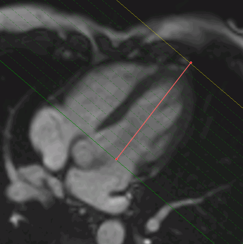
In the window with the LAX merged series, the left ventricle extension is marked with a line (Fig. 8.5).

Figure 8.5: Left ventricle extension shown in the window with the LAX merged series

In multiphase series, the left ventricle extension may be determined for each phase.

8.1.5 Contouring the Left Ventricle Endocardium and Epicardium Automatically

In the Cardiac analysis tab, there are two options for automatic contouring:

contouring is performed in the SAX window on the slices for the selected phases;
contouring is performed in the SAX window on the slices for all the phases.

For automatic contouring of the left ventricle endocardium and epicardium to be performed on the slices for the selected phases, proceed as follows:

Open the study in the Cardiac analysis tab (see Section 8.1.1).
Determine the left ventricle extension (see Section 8.1.4) for the phases where the contouring is to be performed.
Click the Auto contouring button on the toolbar for cardiac function analysis.

Automatic contouring of the left ventricle endocardium and epicardium are performed in the window with the SAX merged series for all the phases with the left ventricle extension and all the slices within the extension. The contour boundaries are shown on the slices in the window with the LAX merged series (Fig. 8.6).

For automatic contouring of the left ventricle endocardium and epicardium to be performed on the slices for all the phases, proceed as follows:

Open the study in the Cardiac analysis tab (see Section 8.1.1).

Determine the left ventricle extension (see Section 8.1.4) for the End Diastole (ED) and End Systole (ES) phases.

If the number of phases for which the left ventricle extension has been determined does not equal two, automatic contouring for all the phases is unavailable. A respective warning will pop up on the screen.

Click the arrow on the right-hand side of the Auto contouring button and select Build all contours based on two phases. The contouring process may take some time.

If you select automatic contouring for all the phases, all the left ventricle contours that were built previously will be deleted.

Automatic contouring of the left ventricle endocardium and epicardium is performed in the window with the SAX merged series for all the phases. The contour boundaries are shown on the slices in the window with the LAX merged series (Fig. 8.6).

Figure 8.6: Automatic contouring of the left ventricle

Attention! If a part of the atrium is present on the mitral valve slice, it may be captures while contouring.

To rebuild all the contours, press the arrow on the right-hand side of the Auto contouring button and select Rebuild contours.

During automatic contouring, it is possible that tissues may be captured by the contour in error. Check that the contours are drawn correctly and edit the contours manually if necessary.

To go to the results of parameters assessment, click the Start analysis button (see Section 8.1.8).

8.1.6 Actions with Contours

The DICOM Viewer provides an opportunity to perform the following actions with contours in the SAX window:

editing. Mouse over the selected contour. When the cursor is placed on the contour, the contour is highlighted. Click the mouse button in the place where you want to edit the contour and build a new contour while holding the mouse button. To complete the contour, release the mouse button;
deleting a contour. Mouse over the selected contour, click the right mouse button, and select the Remove contour option on the context menu;
deleting the extension boundaries. Place the cursor on one of the points used for evaluating the LV extension. The point will be highlighted. Click the right-hand mouse button and select the Remove extension boundaries option on the context menu.

Contours and LV extension boundaries can also be deleted from the contours panel (see Section 8.1.7).

8.1.7 Contours panel

The contours panel (Fig. 8.7) is expanded/minimized with the "Contours panel" button on the cardiac analysis toolbar. By default, the contours panel is expanded.

Figure 8.7: Contours panel

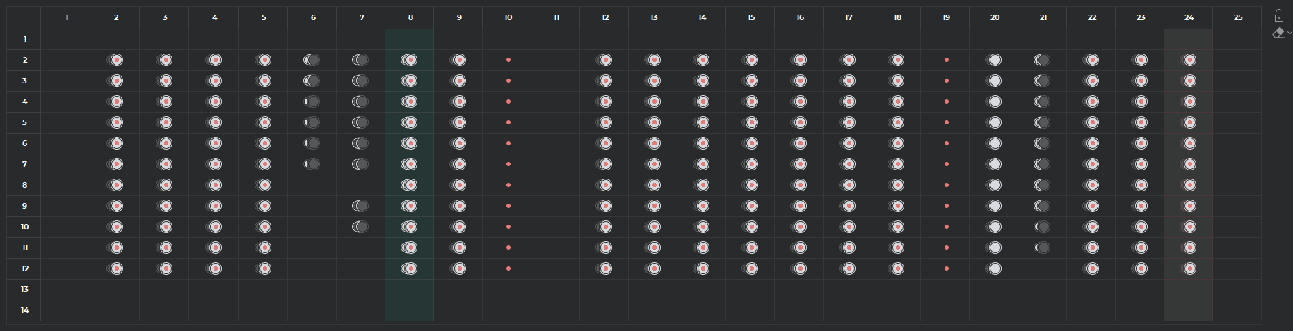
The contours panel provides for navigation between images and for contour management. The contours panel is presented as a phase and slice contingency table. The column header shows the phase number, and the line header shows the slice number. The cells contain information on contours and LV extension boundaries in the form of conventional signs:

endocardial LV contour is ;
epicardial LV contour is ;
endocardial RV contour is ;
epicardial RV contour is ;
LV extension boundaries passage through the slice is .

To go to the selected slice image and phase in the SAX window, left-click on the respective cell. The cell corresponding to the image in the SAX window is highlighted.

The DICOM Viewer provides an opportunity to perform the following actions with contours:

Deleting contours on the selected slice. Right-click on the selected cell and on the context menu, select:
- Remove LV endocardial contour (<slice number; phase number>);
- Remove LV epicardial contour (<slice number; phase number>);
- Remove RV endocardial contour (<slice number; phase number>);
- Remove RV epicardial contour (<slice number; phase number>).
Deleting a certain type of contours on all the images for the selected phase. Right-click on the column header (phase number) and on the context menu, select:
- Remove LV endocardial contours (<phase number>);
- Remove LVepicardial contours (<phase number>);
- Remove RV endocardial contours (<phase number>);
- Remove RV epicardial contours (<phase number>).
In the dialog box that opens, click YES to conﬁrm the deletion, or click NO to cancel.
Deleting a certain type of contours on all the images for the selected slice. Right-click on the line header (slice number) and on the context menu, select:
- Remove LV endocardial contours (<slice number>);
- Remove LV epicardial contours (<slice number>);
- Remove RV endocardial contours (<slice number>);
- Remove RV epicardial contours (<slice number>).
In the dialog box that opens, click YES to conﬁrm the deletion, or click NO to cancel.
Deleting all the contours of the same type. Click the arrow on the right-hand side of the Remove all cardiac contours button. On the menu, select the type of contours you want to delete from all the slices. In the dialog box that opens, click YES to conﬁrm the deletion, or click NO to cancel. The selected contour type is removed from all slices and phases in the SAX window.
Deleting all the contours. To delete all the contours, click the Remove all cardiac contours button. In the dialog box that opens, click YES to conﬁrm the deletion, or click NO to cancel. All the contours on all the slices in the window with the SAX merged series will be deleted.
Deleting LV extension boundaries for the selected phase. Right-click on the column header (phase number) and on the context menu, select: Remove lv extension boundaries (<phase number>).

The program automatically detects and highlights the end phases with the maximum and the minimum ventricle cavity volume at the time of relaxation (diastole) and contraction (systole). The ﬁnal phase of contraction (ES) is highlighted with green, and the ﬁnal phase of relaxation (ED) — with red.

To lock the end phases, click the Lock end phases button on the contours panel. After the end phases are locked, the button will take the shape of . In this case, the end phases cannot be detected automatically after creating, editing, and deleting contours. To enable automatic detection of the end phases, click the Unlock end phases button on the contours panel. The button will take the shape of .

The user may manually set and lock the selected end phase as ES or ED. To do that, right-click on the column header (phase number) and on the context menu, select Set <phase number> as ES or Set <phase number> as ED.

8.1.8 Evaluating Functional Parameters of the Heart

To evaluate functional parameters of the heart, proceed as follows:

Open the study in the Cardiac analysis tab (see Section 8.1.1).
Build the required contours manually or automatically (see Sections 8.1.3 and 8.1.5).
Click the Start analysis button on the toolbar for cardiac function analysis.

The results of functional parameters evaluation and the information on the patient are presented as a table. The following basic parameters for the left and the right ventricle are evaluated:

EDV (end diastolic volume), the maximum ventricle cavity volume at the end of diastole, measured in ml. To evaluate the parameter, you need to build the endocardial contours;
ESV (end systolic volume), the minimum ventricle cavity volume at the end of contraction (systole), measured in ml. To evaluate the parameter, you need to build the endocardial contours;
SV (stroke volume), the volume of blood ejected with each heart beat, measured in ml and calculated by the SV = EDV — ESV formula. To evaluate the parameter, you need to build the endocardial contours;
EF (ejection fraction), the percentage of blood ejected with each heart beat calculated by the EF = SV/EDV formula. To evaluate the parameter, you need to build the endocardial contours;
CO (cardiac output), the amount of blood pumped in a minute, measured in l/min by the CO = SV * heart rate formula. To evaluate the parameter, you need to build the endocardial contours and know the heart rate;
CI (cardiac index), the cardiac output related to the body surface area (BSA). The parameter is measured in and calculated by the CI = CO/BSA formula. The body surface area (BSA) is calculated by the following formula: BSA = 0.007184 ∗ W^0.425 ∗ H^0.725, where W is the patient’s weight in kilos and H is the patient’s height in centimeters. To evaluate the parameter, you need to build the endocardial contours and know the patient’s weight and height;
Myocardial mass, shows the diﬀerence in the epicardium and endocardium volumes at the end of diastole (ED) and systole (ES) multiplied by a factor of 1.05, measured in g. To evaluate the parameter, you need to build the endocardial and epicardial contours for the ED and ES phases.

The results of functional parameters evaluation can be copied to the clipboard and then inserted in the report editor (see Chapter 18) or in any text editor. To copy the results of functional parameters evaluation to the clipboard, click the EXPORT TO CLIPBOARD button.

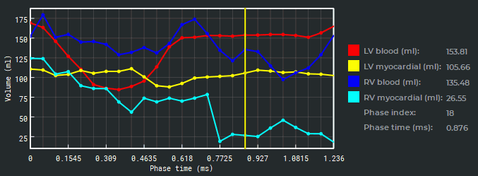
The coordinate system (Fig. 8.8) shows the functional parameters for all the phases as graphs. On the x- axis, you can see the time in milliseconds while on the y- axis the blood volume is shown in milliliters.

Attention! Graphs are built on the basis of the contours created for each slice of each phase in the window with the SAX merged series.

The coordinate system shows the heart functional parameters as graphs:

left ventricle endocardium volume LV blood (red line);
left ventricle myocardium volume LV myocardial (yellow line);
right ventricle endocardium volume RV blood (dark blue line);
right ventricle myocardium volume RV myocardial (light blue line).

The measurement results are shown as a table on the right-hand side of the coordinate plane. The values of the parameters reﬂect the measurement results for the current point.

Figure 8.8: Heart functional parameters shown as graphs

The position of the current phase is marked with the yellow slider. To change the current phase on the graph, mouse over the slider so that the cursor takes the shape. Holding the left mouse button, move the slider to the left or to the right. When you move the slider, the current phase in the window with the SAX merged series is changed simultaneously. When the current phase is changed, the measurement results shown in the table next to the graphs are also changed.

To move the graph along the y-axis, move the mouse up and down while holding the left mouse button and the Shift key on the keyboard. To scale the graph, move the mouse up and down while holding the left mouse button and the Ctrl key (or the Command key for macOS) on the keyboard.

To edit the information on a patient, click the EDIT PATIENT INFO button and make the necessary corrections in the dialog box (Fig. 8.9). Click OK to apply the new data or CANCEL to cancel. After you click the OK button, the results of functional parameters analysis will be reevaluated.

Figure 8.9: Dialog box for editing the information on a patient

To get back to the contour building and editing mode, click the Edit button.

[next] [front] [up]